
Active perception and decentralized decision-making
In this post, I give an overview of my recent research on multi-agent active perception, published in the two recent papers (Lauri et al., 2020; Lauri et al., 2019).
Active perception is a process by which an agent, a software agent or an embodied agent such as a robot, perceives its environment to reduce uncertainty in order to accomplish some task. For instance, a robot that wants to grab a cup from the kitchen table first needs to detect where the cup is, perhaps by moving around the table and capturing images as it goes. Here, the robot is engaging in active perception towards the end goal of grasping the cup.
To put it another way, (Bajcsy et al., 2018) states that
[a]n agent is an active perceiver if it knows why it wishes to sense, and then chooses what to perceive, and determines how, when and where to achieve that perception.
In multi-agent active perception, a team of agents collaboratively engages in active perception. You can think of a group of search and rescue robots attempting to locate victims of a disaster, or a team of exploration rovers collecting scientific samples on the surface of a planet. My recent research concerns the theory of such active perception problems viewed as sequential decision-making tasks. Each agent takes an individual action, and then perceives an individual observation. The agents then select the next action, and the process repeats until termination. We considered a very general case, with the following properties:
- The agents act independently, and there is no implicit communication or information sharing between agents
- The state undergoes a stochastic state transitions conditional on the individual actions of all agents
- The agents do not know the underlying true state of the system, but rather perceive individual observations correlated with the state.
- The objective of the agents is to reduce uncertainty about the hidden state.
Such problems are appropriately modelled as decentralized partially observable Markov decision processes, or Dec-POMDPs. To give a bit of context for our work, I will first review some formalizations of sequential decision-making that underlie planning and reinforcement learning. These are the Markov decision process (MDP), the partially observable MDP (POMDP), and finally the multiagent generalization, the decentralized POMDP (Dec-POMDP). Finally, I will discuss multi-agent active perception modelled as a Dec-POMDP, which the two papers referenced above are all about.
Planning and reinforcement learning formalisms
Markov decision processes formalize decision-making tasks with different kinds of underlying assumptions. Planning and reinforcement learning methods may be applied to solve the decision-making problem.
Full state observability - Markov decision process (MDP)
The basic concepts found in all Markov decision processes are state, action, and reward.
- The state of the system in a Markov decision process is a collection of all features and variables relevant to the problem at hand. For example, the state in a navigation problem might be the position of the agent in the environment.
- The actions are the choices available to the agent. For instance, the navigating agent from above might choose to move east, west, north, or south. Each action typically has some effect on the state: moving east will change the state of the agent so it is more to the east, and so on.
- Finally, rewards encode the task of the agent. The reward depends on the current state and the current action. The greater the reward, the more desirable it is to take the action in the state. The navigating agent’s goal can be described through the reward: it can obtain a large positive reward when it reaches the goal location. On the other hand, the reward can model undesirable states: moving off a cliff ledge will result in a large negative reward.
Interaction of the agent and the system in a MDP proceeds as follows. The system is in some state \(s\) which is known to the agent. The agent then selects an action \(a\) to execute. The agent will obtain a reward \(r \), and the system state will transition to a new state \(s'\). Then the process is repeated in the new state.
The state transitions in a MDP are not deterministic, that is, they cannot always be precisely predicted. As a concrete example, if the agent moves east, it might end in a location exactly to the east with some probability, and with some probability, it will end up in a location that is slightly off from the expected location. The state transitions are assumed to be governed by a transition model \( T(s', a, s)\) that gives the conditional probability of the next state \(s'\) given the current state \(s\) and action \( a\). It is also assumed that the rewards are governed by a reward model \(R(s, a)\) that gives the immediate reward of executing action \(a\) in state \(s\).
The key question in planning and reinforcement learning is how the agent should act in a given state to maximize the expected sum of rewards it can collect over a long time horizon. Rewards that are obtained quickly are considered more valuable than those far in the future. This is modelled by a discount factor \( \gamma\), a number between 0 and 1. Rewards \(k\) steps in the future are discounted by \(\gamma^k\). The question of how to act is answered by a policy that maps states to actions. We denote the policy as a function \(\pi \), and the action selected by the policy in state \(s\) by \(\pi(s) = a\).
How good a policy is is measured by its value. Particularly useful is the concept of an action-value function \(Q^\pi \) of a policy \(\pi\). The action-value function takes as input a state \(s\) and an action \( a\), and returns the expected sum of rewards obtained when first executing action \(a\) in the starting state \(s\), and then acting according to the policy \(\pi\) from there on. The action value function is defined as \begin{equation} Q^{\pi}(s,a) \triangleq \mathbb{E}\left[ R(s_0, a_0) + \sum\limits_{t=1}^{\infty}\gamma^t R(s_t, \pi(s_t)) \middle| s_0 = s, a_0 = a\right]. \end{equation} We can also define the value function of \(\pi\) in a state \( s\) as \begin{equation} V^{\pi}(s) \triangleq \mathbb{E}\left[ \sum\limits_{t=0}^{\infty}\gamma^t R(s_t, \pi(s_t)) \middle| s_0 = s\right]. \end{equation} An optimal policy maximizes the value of every state, that is, a policy \(\pi^*\) is optimal if and only if for every policy \( \pi\) and every state \(s\), \(V^{\pi^*}(s) \geq V^{\pi}(s)\).
In a reinforcement learning (RL) setting, The transition model \(T\) and the reward model \(R\) are not known to the agent. Instead, the agent interacts with the environment, recording a sequence of states, actions, and rewards. In model-free reinforcement learning, the objective is to directly learn the action-value function \(Q^{\pi^*}\) of an optimal policy. In model-based RL, estimate models \(\hat{T}\) and \( \hat{R}\) are learned, and then used to compute an optimal policy. The estimated models are used as a simulator to compute an optimal policy offline, for which no interaction is required. The process of computing an optimal policy from given or estimated models is known as planning.
A famous example of model-free RL is the deep Q network (Mnih et al., 2013) that learns to play Atari games. In this case, the state \(s \) is the last few video frames of the game, and the action-value function \(Q^{\pi}(s,a)\) determines the value of every game action \(a\), such as pushing a button or moving the joystick. The best action to select is determined according to the action-value function as \( a_t = \pi(s_t) = \operatorname{arg max}\limits_{a_t} Q^{\pi}(s_t, a_t)\).
Partial state observability - partially observable MDP (POMDP)
A limitation of the MDP formalization is that the state is assumed to be known to the agent. This is not always the case. For example, in some of the Atari games mentioned above, a few video frames may not be enough to determine the velocity of a moving object. Arguably the velocity of an object is part of the state, so this means that the game-playing agent cannot actually perceive the state from the given input!
In such cases, the state is partially observable. The MDP framework can be changed as follows to account for this. First, the state will be “hidden” from the agent – it can no longer know what the state \( s\) of the system is. Secondly, observations are added to the framework. Observations are correlated with the true underlying state of the system. This is modelled via an observation model \(O(z', s', a)\) that gives the conditional probability of perceiving observation \( z'\) given the state \(s'\) and the previous action \( a\). As before, in an RL setting, \(O \) along with the transition model \( T\) and reward model \( R\) are not known to the agent. These two changes give the partially observable MDP (POMDP). There is a price to pay for the added expressiveness of the POMDP model, however, as we shall see next.
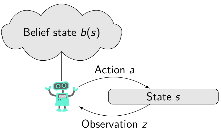
As the state is no longer observable, the experiences of the agent are now sequences of actions, rewards and observations. That is, an experience of length-\(t \) is a sequence \(h_t = (a_0, r_0, z_1, a_1, r_1, z_2, \ldots, a_{t-1}, z_t ) \). The sequence \(h_t\) is also called a history of actions and observations.
The policy \(\pi\) also has to be changed: since the agent does not know \( s\), a policy of the form \(\pi(s) = a\) is no longer viable. Instead, the policy should map histories to the next action: \( \pi(h_t) = a_t \). This presents a problem. As time goes on, the size of the history \(h_t \) increases. Soon, it will become infeasible to store the history, let alone represent a policy function that maps any possible history to an action!
The solution to the problem is to summarize the history \(h_t \) into some fixed-size representation \( b_t\).
In model-free RL, this is nowadays often done by applying a recurrent neural network such as a long-short-term memory (LSTM) unit. The internal state of the LSTM is used as the summary \(b_t\). The LSTM \(f\) is then used to update the internal representation given a new action \(a_t\) and a new observation \(z_{t+1}\): \(b_{t+1} = f(b_t, a_t, z_{t+1})\). In model-based RL and planning, the summary \(b_t\) is defined as the belief state, a probability over the state \(s_t\) given the history \(h_t\): \(b_t(s_t) \triangleq \mathbb{P}(s_t \mid a_0, z_1, \ldots, a_{t-1}, z_t)\). The estimated models \( \hat{T}\) and \( \hat{O}\) are applied to compute the updated \(b_{t+1}\) by applying Bayesian filtering. Given the previous belief state \(b_t\) and a new action \(a_t\) and a new observation \(z_{t+1}\), the updated belief for state \(s_{t+1}\) is \begin{equation} b_{t+1}(s_{t+1}) \triangleq \eta \hat{O}(z_{t+1}, s_{t+1}, a_t) \sum\limits_{s_t}\hat{T}(s_{t+1},a_t,s_t)b_t(s_t), \end{equation} where \(\eta\) is a normalization factor.
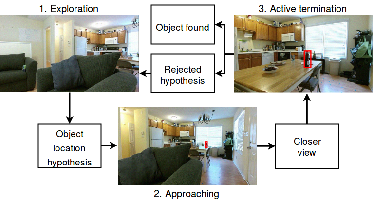
Since \(b_t\) is now a fixed-size summary of the history, it is possible to represent the action-value function \(Q^{\pi}(b_t, a_t)\), and apply it much in the same way as in the MDP case to select actions. A good example of this is the deep recurrent Q network (DRQN) (Hausknecht & Stone, 2015), that was again applied to play Atari games. We also applied the DRQN to the problem of active visual object search in (Schmid et al., 2019). The hidden state is the location of the target object, while the agent’s observations are the images it can see from its current location. The actions of the agent are the different movement actions, and some special actions that declare the object to be found (active termination). Positive rewards are accrued for successfully finding the target object, while negative rewards are accumulated for false declarations and movements.
Multiple agents - decentralized POMDP (Dec-POMDP)
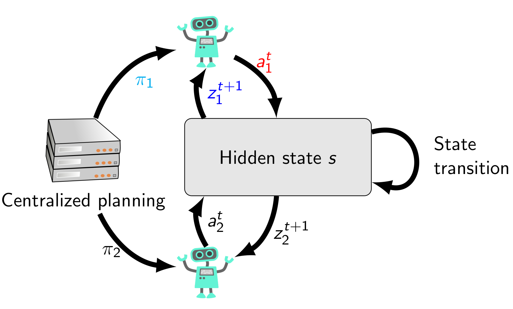
Now we have gone from the MDP to the POMDP by hiding the state from the agent, and by adding observations. The decentralized POMDP (Dec-POMDP) is a generalization of a POMDP with multiple cooperating agents. For simplicity, I will consider here the case with two agents, but the Dec-POMDP is applicable to any finite number \(n\) of agents. For an in-depth introduction to Dec-POMDPs, I recommend the book by Oliehoek and Amato (Oliehoek & Amato, 2016).
Both agents are independent in the sense that they take their own individual actions, and perceive their own individual observations. Therefore, they experience an individual history, and have individual policies. The system state transitions, observations, and rewards however still depend on the joint actions of the agents. A joint action is a tuple \(a_t = \langle a_{1,t}, a_{2,t}\rangle\) of both agents’ individual actions \(a_{i,t}\). The transition model is defined on these joint actions, that is, \begin{equation} T(s_{t+1}, a_t, s_t) = T(s_{t+1}, a_{1,t}, a_{2,t}, s_t) \end{equation} gives the conditional probability of the next state being \(s_{t+1}\) when the agent 1 takes an individual action \( a_{1,t}\), and agent 2 takes an individual action \( a_{2,t}\), and the previous state is \( s_t\). Similarly, a joint observation is a tuple \( z_t = \langle z_{1,t}, z_{2,t} \rangle\) of individual observations \(z_{i,t}\). The observation model defines the conditional probability of a joint observation given the state and the previous joint action: \begin{equation} O(z_{t+1}, s_{t+1}, a_t) = O(z_{1,t+1}, z_{2,t+1}, s_{t+1}, a_{1,t}, a_{2,t}). \end{equation} The rewards in a Dec-POMDP are shared. The reward model is defined \begin{equation} R(s_t, a_t) = R(s_t, a_{1,t}, a_{2,t}), \end{equation} determining the reward of taking joint action \(a_t = \langle a_{1,t}, a_{2,t}\rangle\) in state \(s_t\).
One agent does not know precisely how the other agent acted, or what the other agent perceived. Each agent has its own individual history \(h_{i,t} = (a_{i,0}, z_{i,1}, \ldots, a_{i,t-1}, z_{i,t})\). Therefore, the individual policy of each agent maps individual histories to actions: \( \pi_{i}(h_{i,t}) = a_{i,t}\). A joint policy is a tuple of individual policies, that is \( \pi = \langle \pi_1, \pi_2 \rangle\). Because information is not shared, it is not possible anymore to come up with a single global summary \(b_t\) of the hidden state as in the POMDP. Instead, each agent can either remember its individual history, or create an individual summary \( b_{i,t}\) of it.
The paradigm of centralized planning, decentralized execution is assumed in Dec-POMDPs. Individual policies of each agent are designed in a centralized manner, but they can be executed by each agent independently, without knowing what the other agents are doing. This means that we can reason about the joint summary \(b_t\) of the agents during planning, even if no individual agent has the capability to compute this summary at execution-time. This reasoning is the key part of multi-agent active perception modelled as a Dec-POMDP.
Multi-agent active perception
In some active perception problems there is a clear state-based objective. These types of problems can be thought of as active hypothesis testing. For example in the active visual object search example discussed earlier, there is a set of competing hypotheses (possible locations of the target object), and the agent is trying to discriminate between these objectives. The agent is rewarded for successfully declaring the correct hypothesis, and penalized for mistakes or taking too much time.
However, some active perception problems are more open-ended, or curiosity driven. Consider for example a monitoring task, like the task of monitoring ocean currents. There is no state-based objective or desirable state to reach – the currents are what they are and change over time – so there is no right hypothesis to call. Instead, the objective would be to reduce uncertainty about the hidden state in the problem. These types of active perception problems are exactly the type we consider in a multi-agent setting in (Lauri et al., 2020; Lauri et al., 2019).
We modify the reward function of the problem, so that it is not dependent on the state, but rather on what the agents know about the state, that is, the summary or belief state \(b_t\) discussed earlier. Uncertainty of a belief state can be quantified by using the information entropy. Recall the belief state \(b_t\) defined as a probability over possible hidden state \(s_t\). The entropy of the belief state is \begin{equation} H(b_t) \triangleq -\sum\limits_{s_t}b_t(s_t) \ln b_t(s_t). \end{equation} Applying the negative entropy as a reward function makes the agents prefer policies that are likely to lead to a belief state with low uncertainty.
We were able to derive some useful theoretical results for these types of active perception problems in the multi-agent setting. We established that the action-value function \(Q^{\pi}(b_t,a_t)\) and the value function \(V^{\pi}(b_t)\) of any joint policy \( \pi \) are convex functions of the belief state \(b_t\). This lead to a practical algorithm for planning policies for active perception.
For our algorithm, we chose to represent individual policies as finite state controllers, or policy graphs, as shown in the figure below. Each agent starts executing a fixed-size policy graph from an initial controller node shown on the left hand side of the respective figures. Then, the agent takes the action read from the table for the controller node. The individual observation perceived by the agent then determines what is the next controller node it transitions to: this is modelled by the edges of the policy graph. This approach produces compact and easily understandable policies, while also limiting the search space.
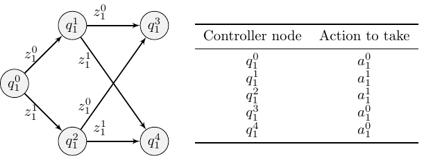
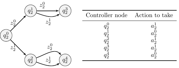
The core idea of our planning algorithm is to iteratively improve the policy graphs. Improvements are done by 1) changing the individual action to be taken at a controller node, and 2) changing the out-edge configuration of a controller node. If we are improving a node, say, \(q_1^1\), we answer questions such as: “if agent 1 is in controller node \(q_1^1 \), what are the probabilities of the possible controller nodes where agent 2 is?”. Then, we also consider the belief states in a similar manner: “if agent 1 is in controller node \(q_1^1\) and agent 2 is in controller node \(q_2^2 \), what are the possible belief states and what are their relative likelihoods?”. Using this information, we are able to calculate if changing the individual action or where out-edges are connected to at node \(q_1^1\) would result in a greater expected value for the joint policy.
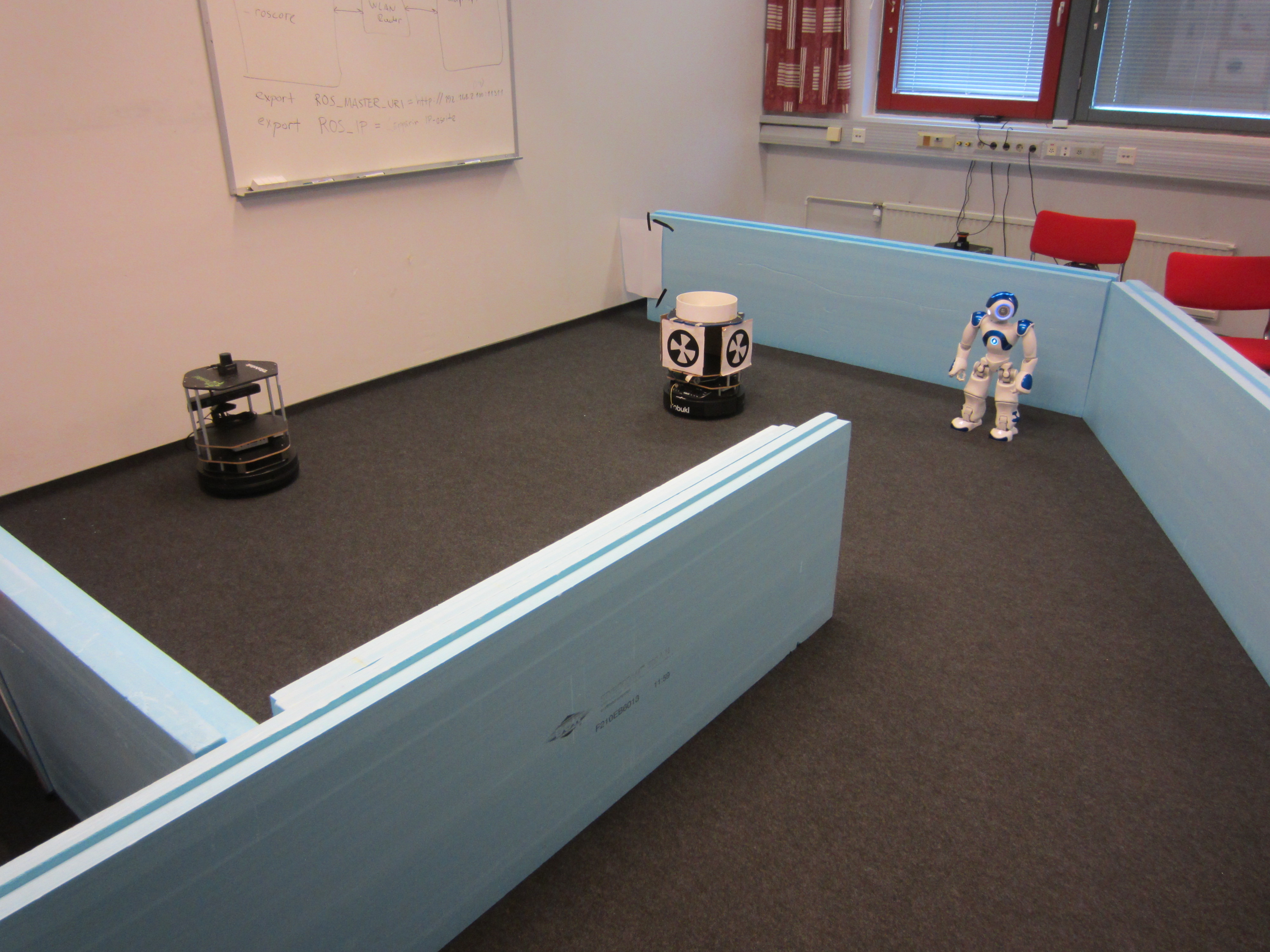
We applied the algorithm to two multi-agent active perception problems. In one of the problems, two micro air vehicles (MAVs) are tracking a moving target. The target is either friendly or hostile. A hostile target will tend to move quickly in order to avoid detection, while a friendly target tends to move more slowly. The two MAV agents can either use a camera or radar to detect the target. The camera is reliable on short ranges, but does not work well with a longer range. The radar in turn works well with long ranges to the target, but if both MAVs use their radar simultaneously the accuracy suffers due to interference. The camera and radar measurements only provide information about the location of the target. The type (friendly or hostile) of the target must be inferred from a longer sequence of observations, tracking the behaviour of the target. In earlier work (Lauri et al., 2017), we applied a similar model to a real-world problem of two robots tracking a target, as shown in the image below.
Using our proposed algorithm, we were able to find efficient and compact individual tracking policies . By using particle filtering to track the belief state, we could extend the algorithm to the case where the hidden state \(s_t\) is continuous, while the actions and observations are discrete. We demonstrated this variant of the algorithm in a signal source localization task in (Lauri et al., 2020).
If you are interested in trying out this algorithm for yourself, either to solve multi-agent active perception problems or regular Dec-POMDPs, you can find the code on Github.
The limitations of our algorithm are discussed in (Lauri et al., 2020). Firstly, at each improvement round we need to compute all belief states reachable under the current policy. This requires a lot of memory, which will limit the scalability of the algorithm. Secondly, the size of the policy graph has to be fixed beforehand. Choosing a too small policy graph might prevent finding good policies, while using a too large policy graph will waste computational resources. Finally, because the reward function depends on the belief state and not the state, we have to use a Bayes filter to compute belief states at planning time. As a result, the scale of the problems that can currently be solved is not quite up to par with state-of-the-art solvers for Dec-POMDPs with state-based rewards. The algorithm we proposed is heuristic – although it performed well experimentally, it does not provide any performance guarantees compared to an optimal solution. These are among some of the issues we hope to address in future work.
Conclusion
This post gives a brief overview of different variants of Markov decision processes and how they are used as underlying formalisms for reinforcement learning and planning. In active perception problems, an agent or a team of agents perceive the world to achieve some goal state or simply to reduce uncertainty in their knowledge of the state. Using a decentralized partially observable Markov decision process (Dec-POMDP) as an underlying framework, it is possible to define very general multi-agent active perception problems. No implicit information sharing is assumed, the underlying state is only partially observable, while the system undergoes stochastic state transitions.
Our recent research provides some theoretical grounding for multi-agent active perception as a Dec-POMDP, and proposes the first heuristic algorithm for solving such problems. As discussed above, the approach is not without limitations. I believe there are many further properties of Dec-POMDPs for multi-agent active perception to be discovered. These will hopefully lead to even more powerful solution algorithms as well.
References
- Lauri, M., Pajarinen, J., & Peters, J. (2020). Multi-agent active information gathering in discrete and continuous-state decentralized POMDPs by policy graph improvement. Autonomous Agents and Multi-Agent Systems, 34(42). https://doi.org/10.1007/S10458-020-09467-6[DOI] [Code] [Show/hide BibTeX] [Copy BibTeX to clipboard]
- Lauri, M., Pajarinen, J., & Peters, J. (2019). Information Gathering in Decentralized POMDPs by Policy Graph Improvement. Proceedings of the 18th International Conference on Autonomous Agents and Multiagent Systems (AAMAS), 1143–1151. https://dl.acm.org/doi/abs/10.5555/3306127.3331815[URL] [arXiv] [Code] [Show/hide BibTeX] [Copy BibTeX to clipboard]
- Bajcsy, R., Aloimonos, Y., & Tsotsos, J. K. (2018). Revisiting active perception. Autonomous Robots, 42(2), 177–196.[Show/hide BibTeX] [Copy BibTeX to clipboard]
- Mnih, V., Kavukcuoglu, K., Silver, D., Graves, A., Antonoglou, I., Wierstra, D., & Riedmiller, M. (2013). Playing atari with deep reinforcement learning. ArXiv Preprint ArXiv:1312.5602.[Show/hide BibTeX] [Copy BibTeX to clipboard]
- Hausknecht, M., & Stone, P. (2015). Deep recurrent Q-learning for partially observable MDPs. 2015 AAAI Fall Symposium Series.[Show/hide BibTeX] [Copy BibTeX to clipboard]
- Schmid, J. F., Lauri, M., & Frintrop, S. (2019, November). Explore, Approach, and Terminate: Evaluating Subtasks in Active Visual Object Search Based on Deep Reinforcement Learning. IEEE/RSJ Intl. Conf. on Intelligent Robots and Systems (IROS). https://doi.org/10.1109/IROS40897.2019.8967805[PDF] [DOI] [Code] [Video] [Show/hide BibTeX] [Copy BibTeX to clipboard]
- Oliehoek, F. A., & Amato, C. (2016). A Concise Introduction to Decentralized POMDPs. Springer.[Show/hide BibTeX] [Copy BibTeX to clipboard]
- Lauri, M., Heinänen, E., & Frintrop, S. (2017). Multi-Robot Active Information Gathering with Periodic Communication. IEEE Intl. Conf. on Robotics and Automation (ICRA), 851–856. https://doi.org/10.1109/ICRA.2017.7989104[DOI] [arXiv] [Show/hide BibTeX] [Copy BibTeX to clipboard]