
Multi-robot next-best-view planning
In this post, I give an overview of my recent paper (Lauri et al., 2020) on multi-robot next-best-view planning.
Robots need three-dimensional scene models for many tasks ranging from manipulation to mapping and motion planning. To build a scene model, the robot needs to collect data, for example depth images of point clouds, from many different viewpoints. These data are then fused together to create the scene model in a process known as scene reconstruction.
Next-best-view (NBV) planning refers to intelligently choosing how and where the robot should capture the next images. The objective is to reduce the time and resources required to obtain a scene reconstruction of sufficient quality. Single-robot NBV planning therefore often considers utility functions such as the expected information gain available from a particular view.
When multiple robots are used for scene reconstruction, the robots should coordinate their actions. They should avoid views that overlap strongly, because that is inefficient. NBV planning for multiple robots therefore needs to consider not only the information gain for a single robot, but for the team of robots as a whole, as illustrated in the figure below.
Let us assume we have a team of \(n\) robots performing scene reconstruction. Each robot \( i = 1, 2, \ldots, n \) may choose its next view \(x_i\) from some set \(X_i \) of potential views. The utility of selecting this set of views is measured by a utility function \(f \) that maps tuples of views to a real number proportional to “how good” these views are. The NBV planning problem can be stated as a maximization problem \begin{equation} \max\limits_{\forall i: x_i \in X_i} f(x_1, x_2, \ldots, x_n), \end{equation} that is, maximize the utility over all possible valid choices of views for each robot.
In our recent paper (Lauri et al., 2020) we make two contributions to solving these kinds of multi-robot NBV planning problems:
- We show that a utility function \(f\) can be designed which encourages the robots to avoid selecting overlapping views. Furthermore, this utility function turns out to be a monotonically increasing and submodular function.
- A simple polynomial-time, greedy algorithm can solve the maximization problem above with bounded error, that is, the solution found by the greedy algorithm is withing a constant factor from an optimal solution.
In this post, I describe the technical background of our results, the implementation of the optimization algorithm we used, along with some thoughts about future work that still remains to be done.
Background
Before jumping into solving multi-robot NBV planning problems, we look at two mathematical concepts that enable our results: matroids and submodularity.
Matroids
Matroids generalize the notion of independence from vectors to sets. A matroid \( (\Omega, \mathcal{I})\) consists of a ground set \( \Omega\) and a family of independent sets \( \mathcal{I}\). Every element \( I \in \mathcal{I} \) is an independent set, and is a subset of the ground set. Matroid also need to satisfy a few other properties, a more complete discussion may be found in (Oxley, 2003) or a textbook on the subject.
In our case, the ground set is the union of all robots’ views, that is, \( \Omega = \bigcup\limits_{i=1}^n X_i\). The purpose of the matroid is to represent all valid views selectable by the team of robots by constraining the ground set. In particular, only subsets of \( \Omega\) that contain at most one view per robot are valid. Formally, this leads to the family of independent sets \begin{equation} \mathcal{I} = \left\lbrace I \subseteq \Omega \middle| \forall i: |X_i \cap I| \leq 1 \right\rbrace. \end{equation} This is also known as a block matroid.
The block matroid \( (\Omega, \mathcal{I})\) therefore depicts all valid view combinationss, where each robot chooses either no view at all or a single view. The maximization problem from above can be stated as a matroid-constrained maximization problem \begin{equation} \max\limits_{I \in \mathcal{I}} f(I). \end{equation} Next, we look at a property of the utility function \(f \) that makes this problem easy to approximate.
Submodularity
The utility function \(f\) above maps a tuple of views to a real number. Equivalently, we can think of it as a set function \(f: 2^{\Omega} \to \mathbb{R} \) that maps subsets of the ground set \( \Omega\) to a real number. Here, \(2^\Omega\) denotes the power set of \( \Omega\) – the set of all subsets of \(\Omega\).
Submodularity is an interesting property of set functions. It can be thought of as a diminishing returns property: adding a new element \(x \in \Omega \) to a subset \(A \subset \Omega\) improves the value of \(f\) more the smaller the subset is. Submodularity appears in many applications, for example in sensor placement (Krause et al., 2008). Suppose you are considering deploying a new sensor. Intuitively, if you already have deployd tons of other sensors, the marginal utility of adding this new sensor is not as great compared to if you only have a few sensors so far. Submodularity formalizes this intuition.
Given a set function \(f\), it is submodular if for any \( A \subset B \subset \Omega\) and any \( x \in \Omega \setminus B \), \(f(A \cup \{x\}) - f(A) \geq f(B \cup \{x\}) - f(B)\). Further, \(f\) is said to be monotonically increasing, if for any \(A \subset \Omega \) and \( x \in \Omega \setminus A\), \(f(A \cup \{x\}) \geq f(A)\).
Maximizing a monotonically increasing submodular function
Let’s consider a greedy algorithm for solving the maximization problem \(\max\limits_{I \in \mathcal{I}} f(I)\). Start with the solution \(I_0 = \emptyset\). Then, at steps \(k = 1, \ldots, n \),
- Find the element \(x^* \in \Omega\) that maximizes the marginal utility \(f(I_{k-1} \cup \{x^*\}) - f(I_{k-1})\) such that \( I_{k-1} \cup \{x^*\}\) still satisfies the matroid constraint, that is, \(I_{k-1} \cup \{x^*\} \in \mathcal{I} \)
- Assign \(I_k = I_{k-1} \cup \{x^*\}\) and if \(k < n\), incremnent \(k\) and go back to 1, otherwise return \(I_k\).
If \(f\) is monotonically increasing and submodular, then the solution \(I_n\) returned by this simple greedy algorithm is a bounded approximation. Specifically, it is within a factor of \( \frac{1}{2}\) from the optimal solution: \(f(I_n) \geq \frac{1}{2} \max\limits_{I \in \mathcal{I}} f(I) \). A proof of this result is in (Fisher et al., 1978). This is interesting for many applications where submodularity appears, because a polynomial-time algorithm can be guaranteed to provide a bounded approximation to the overall optimization problem.
Multi-robot next-best-view planning
What remains to be done is to come up with a utility function \(f \) that is suitable for multi-robot NBV planning, and is submodular and monotonically increasing. Then, we can use greedy maximization to solve multi-robot NBV planning problems.
Assumptions
We make two assumptions about the problem at hand. Firstly, we assume the robots can communicate to coordinate their next sensing actions. This is reasonable in settings where the robots are deployed in close proximity with reliable communication, e.g., industrial robots on the same wired network in a warehouse. The problem we consider is therefore a centralized optimization problem. However, the same kinds of methods can also be applied to distributed problems where the robots do not constantly communicate, see for example (Corah & Michael, 2019). Secondly, we assume the potential views of each robot have already been determined, that is, the sets \(X_i\) are known and fixed.
Utility function
In the paper we propose an overlap-aware utility function for multirobot NBV planning. This utility function is based on applying raytracing in the current scene reconstruction to find out which views are likely to result in a high information gain. Overlap is avoided by not rewarding the robots multiple times for observing the same part of the scene.
We use an OctoMap to model the environment as a three-dimensional voxel grid. The OctoMap package already provides tools for raytracing, which makes working with it very convenient in this case. Let’s say there are three robots, and we wish to evalute the usefulness of them selecting the views \(x_1, x_2, x_3 \), respectively. This situation is conceptually illustrated in the figure below. The view \(x_i\) of each robot consists of rays \(r_{i,j}\) that pass through some voxels. These rays indicate the part of the environment potentially seen by each robot, and is illustrated by the shaded voxels.
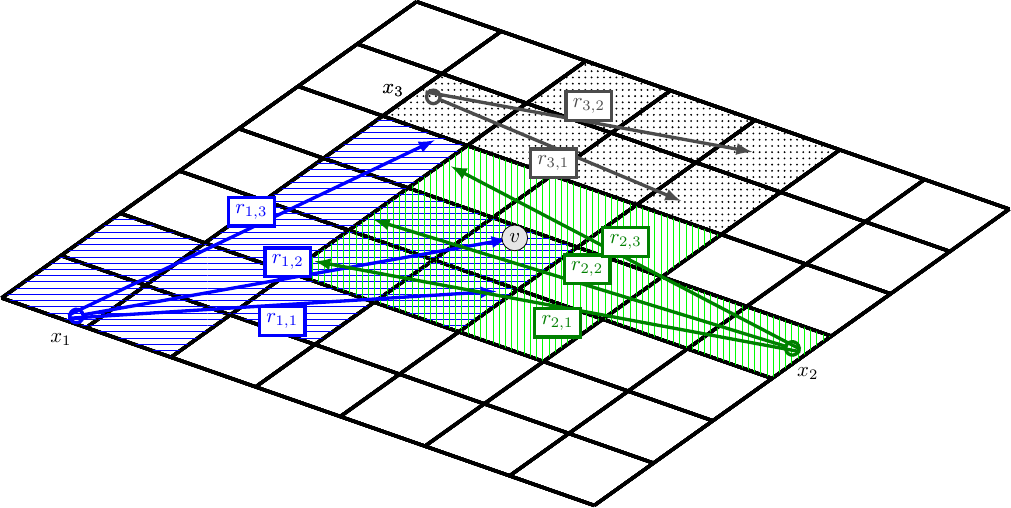
In the example above, views \(x_1\) and \(x_2\) both observe the same voxel \(v\) indicated in the figure – this is not very useful! Even one robot seeing the voxel is sufficient, while the other could use its camera to look elsewhere. Taking this into account is the key feature of our overlap-aware utility function. Informally, our utility function satisfies the following:
For each voxel \(v\) in the environment, the robots gain utility only once, and observing the same voxel from multiple views is not useful.
In the example above, out of all views that could possibly observe \(v\), only the best one is considered by our utility function.
In the paper (Lauri et al., 2020), we prove that our overlap-aware utility function is a monotonically increasing and submodular function. As we saw earlier, maximization problems involving submodular functions are approximately solvable by a greedy algorithm. What is also interesting is that the our utility function generalizes several other utility functions proposed for the single-robot case (Delmerico et al., 2018), helping justify why the greedy optimization strategy is also appropriate in single-robot settings.
Greedy maximization for next-best-view planning
Our proposed utility function can be separated into a sum of per-voxel utilities \(g_v(I)\), where \( v \) is a voxel and \(I\) is an independent set of views. This separation property also makes it easy to implement the greedy maximization algorithm for NBV planning, similar to the one outlined earlier. The algorithm has an initialization stage, which is the only step where costly raytracing is required. After the initialization stage, the maximization can be done simply by querying data from a lookup table.
In the initialization stage, we process for each robot \(i\) each of its candidate views \(x_i \in X_i\). By raytracing, we can determine the subset of voxels that is potentially visible at view \(x_i\). For all such voxels \(v\), we save the per-voxel utility \(g_v(x_i)\) into a data structure.
When we want to find an independent set \( I \) that maximizes the utility \(f\), we proceed similar to the simple greedy algorithm earlier. First, we choose the view \(x\) that has the greatest sum of per-voxel utilities \( g_v(x)\) over all potentially visible voxels. Notice that there is no subscript \(i\) as the view \(x\) could be for any of the robots. Our initial independent set is \( I_1 = \{ x \}\). The per-voxel utility of the independent set \(I_1 \) is initialized to \(g_v(I_1) = g_v(x) \).
At any subsequent step \(k \), we have an independent set \(I_k\). We then process the views of all robots \( i\) whose views are not yet in \(I_k\). We calculate the marginal utility of view \( x_i\) as follows. First we initalize the marginal utility \(M(x_i)\) to zero. We loop over all visible voxels \(v\) at \(x_i\). For each such voxel, there are two possibilities.
- The voxel was not seen by any view so far. Then we add \(g_v(x_i)\) to \(M(x_i)\).
- The voxel was seen by at least one view in \(I_k\). If \(g_v(x_i) > g_v(I_k) \), the new view is better for observing \(v\), and we add \(g_v(x_i) - g_v(I_k)\) to \(M(x_i)\). Otherwise, the old views are better and we do not add anything to \(M(x_i)\).
Finally, we select the view \(x\) that has the greatest marginal utility \(M(x)\) and add it to \(I_k \) to obtain \(I_{k+1}\). The process is repeated until \(k = n\), and we have a view planned for each robot.
How well does it work?
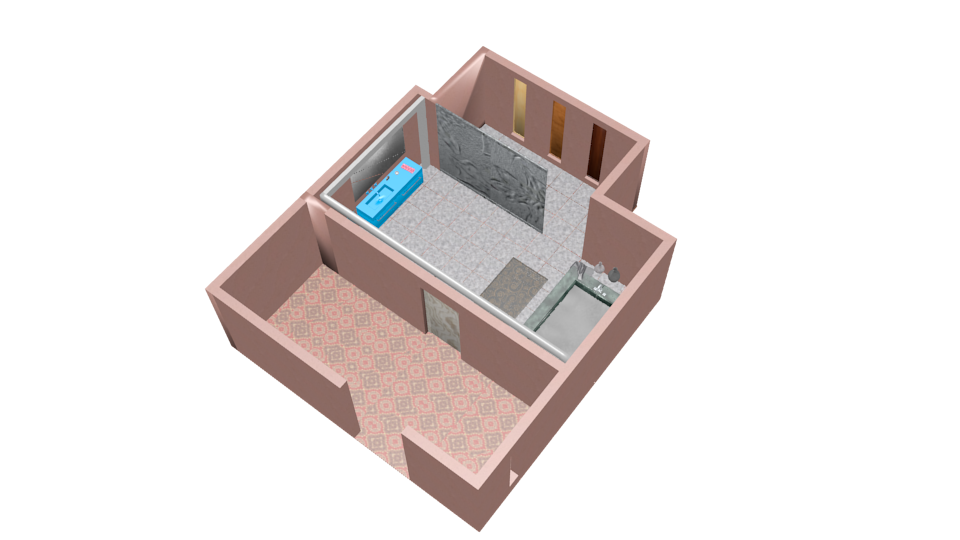
We evaluated the greedy algorithm for multi-robot NBV in simulated and real-world scene reconstruction tasks with multiple robots. The figure below shows an example of two simulated environments we experimented with. In addition to what is shown in the figures, randomly sampled furniture and other objects were present in the simulations. We used scenes from SceneNet RGBD and applied OctoMap for the map representation and raytracing tasks. The single-robot volumetric mapping ROS package also provided a lot of inspiration for the implementation.
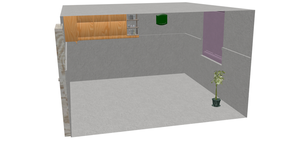
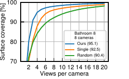
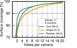
We compared our multi-robot NBV algorithm to randomly selecting views and to planning for each robot separately (ignoring coordination of view planning, leading to more overlap). We measured the surface coverage percentage as a function of the number of views taken by each of 8 robots in the environment. The results are summarized in the plot below, showing that our method works better than the baselines. Bathroom 8 consists of many rooms with occluders, so planning is more important and effective here. This is reflected in the good performance of our method compared to random planning. Kitchen 11 is a single room with no occluding walls, and here the baseline methods also work well as the reconstruction task overall is easier.
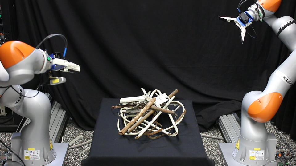
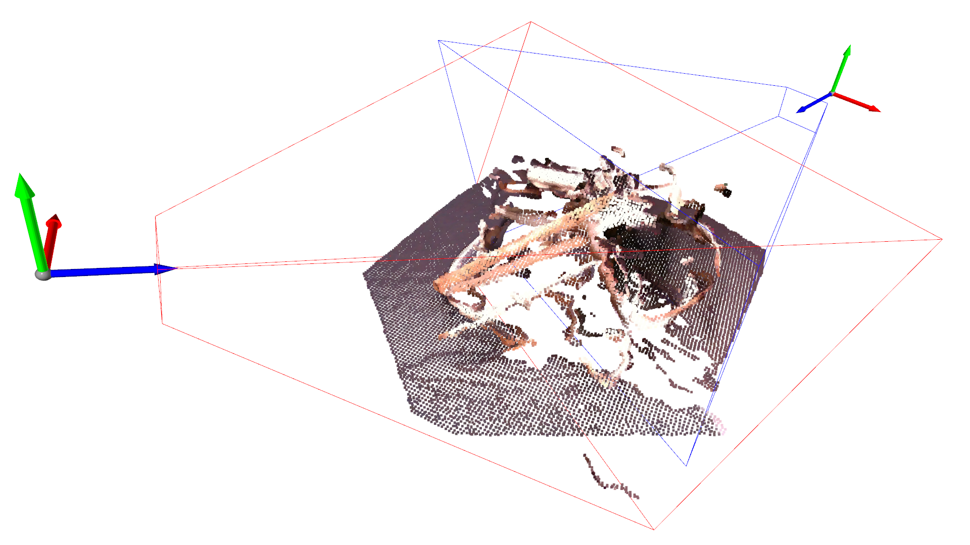
We also deployed our method to a setting with two real robots, as shown in the images at the top of this post. Planning with our utility function that takes overlap into account also worked well in this setting.
Conclusion and future work
In (Lauri et al., 2020) we proposed an overlap-aware utility function for next-best-view (NBV) planning that is applicable to multi-robot settings. There are several interesting directions of future work that we did not explore yet.
- We used a fixed set of candidate viewpoints. The trade-off between having more viewpoints and increased computational time is not clear yet. It might also be useful to create the candidate viewpoints dynamically, instead of working with fixed sets \(X_i\) of views for each robot.
- As mentioned earlier, many utility functions have been proposed for single-robot NBV planning (Delmerico et al., 2018). Our overlap-aware utility function generalizes several of these, but we did not study in detail which utility functions might be most useful for which multi-robot application.
- We also did not tune the parameters of our algorithm in detail, so it remains to be investigated how for example the number of candidate views, raytracing resolution, voxel map resolution, etc., should be set for various applications.
- Constant communication is assumed in the centralized setting. However, matroid-constrained submodular maximization is also applicable with less restrictive centralization assumptions (Corah & Michael, 2019), potentially applicable to NBV planning as well.
I am hoping future research will shed a light on these issues as well!
References
- Lauri, M., Pajarinen, J., Peters, J., & Frintrop, S. (2020). Multi-Sensor Next-Best-View Planning as Matroid-Constrained Submodular Maximization. IEEE Robotics and Automation Letters, 5(4), 5323–5330. https://doi.org/10.1109/LRA.2020.3007445[DOI] [arXiv] [Show/hide BibTeX] [Copy BibTeX to clipboard]
- Oxley, J. (2003). What is a Matroid? CUBO, A Mathematical Journal, 5(3), 176–215.[Show/hide BibTeX] [Copy BibTeX to clipboard]
- Krause, A., Singh, A., & Guestrin, C. (2008). Near-optimal sensor placements in Gaussian processes: Theory, efficient algorithms and empirical studies. Journal of Machine Learning Research, 9(Feb), 235–284.[Show/hide BibTeX] [Copy BibTeX to clipboard]
- Fisher, M. L., Nemhauser, G. L., & Wolsey, L. A. (1978). An analysis of approximations for maximizing submodular set functions – II. In Polyhedral combinatorics (pp. 73–87). Springer.[Show/hide BibTeX] [Copy BibTeX to clipboard]
- Corah, M., & Michael, N. (2019). Distributed matroid-constrained submodular maximization for multi-robot exploration: Theory and practice. Autonomous Robots, 43(2), 485–501. https://doi.org/10.1007/s10514-018-9778-6[DOI] [Show/hide BibTeX] [Copy BibTeX to clipboard]
- Delmerico, J., Isler, S., Sabzevari, R., & Scaramuzza, D. (2018). A comparison of volumetric information gain metrics for active 3D object reconstruction. Autonomous Robots, 42(2), 197–208. https://doi.org/10.1007/s10514-017-9634-0[DOI] [Show/hide BibTeX] [Copy BibTeX to clipboard]